Metran practical example

This notebook shows a practical application of Metran on calculated residuals from univariate time series models as published in the article van Geer and Berendrecht in Stromingen (2015).

[1]:

import os

import pandas as pd

import metran

metran.show_versions()

Python version: 3.10.12 | packaged by conda-forge | (main, Jun 23 2023, 22:40:32) [GCC 12.3.0]
numpy version: 1.26.4
scipy version: 1.12.0
pandas version: 2.2.0
matplotlib version: 3.7.2
pastas version: 1.4.0
numba version: 0.59.0
lmfit version: 1.2.2

Read example data

Read residuals from time series analysis models for 5 piezometers at different depths at location B21B0214. (The time series models are not shown here, only the resulting residuals.)

[2]:

residuals = {}
rfiles = [
    os.path.join("./data", f) for f in os.listdir("./data") if f.endswith("_res.csv")
]

for fi in rfiles:
    name = fi.split(os.sep)[-1].split(".")[0].split("_")[0]
    ts = pd.read_csv(
        fi, header=0, index_col=0, parse_dates=True, date_format="%Y-%m-%d"
    )
    residuals[name] = ts

[3]:

# sort names (not necessary, but ensures the order of things)
sorted_names = list(residuals.keys())
sorted_names.sort()
sorted_names

[3]:

['B21B0214001', 'B21B0214002', 'B21B0214003', 'B21B0214004', 'B21B0214005']

Create Metran model

First collect series in a list with their unique IDs.

[4]:

series = []

for name in sorted_names:
    ts = residuals[name]
    ts.columns = [name]
    series.append(ts)

Create the Metran model and solve.

[5]:

mt = metran.Metran(series, name="B21B0214")
mt.solve()

INFO: Number of factors according to Velicer's MAP test: 1


Fit report B21B0214                  Fit Statistics
=======================================================
tmin     None                        obj        2332.33
tmax     None                        nfev            77
freq     D                           AIC        2344.33
solver   ScipySolve

Parameters (6 were optimized)
=======================================================
                         optimal   stderr initial  vary
B21B0214001_sdf_alpha   5.501017  ±18.98%    10.0  True
B21B0214002_sdf_alpha  13.560042  ±10.04%    10.0  True
B21B0214003_sdf_alpha   4.682870  ±28.86%    10.0  True
B21B0214004_sdf_alpha  11.381674  ±18.22%    10.0  True
B21B0214005_sdf_alpha  13.140605   ±8.48%    10.0  True
cdf1_alpha             22.980925   ±7.43%    10.0  True

Parameter correlations |rho| > 0.5
=======================================================
None

Metran report B21B0214        Factor Analysis
=============================================
tmin     None                nfct     1
tmax     None                fep     88.32%
freq     D

Communality
=============================================

B21B0214001      73.61%
B21B0214002      87.59%
B21B0214003      93.35%
B21B0214004      91.74%
B21B0214005      81.15%

State parameters
=============================================
                      phi         q
B21B0214001_sdf  0.833781  0.080429
B21B0214002_sdf  0.928908  0.017023
B21B0214003_sdf  0.807716  0.023102
B21B0214004_sdf  0.915889  0.013316
B21B0214005_sdf  0.926724  0.026607
cdf1             0.957419  0.083349

Observation parameters
=============================================
                   gamma1     scale      mean
B21B0214001      0.857982  5.920523 -0.001924
B21B0214002      0.935874  5.565866 -0.055813
B21B0214003      0.966197  5.702295 -0.001265
B21B0214004      0.957794  5.833851 -0.033373
B21B0214005      0.900857  6.234234 -0.022840

State correlations |rho| > 0.5
=============================================
None

Visualizing and accessing Metran results

The results of the Metran can be visualized using the Metran.plots class.

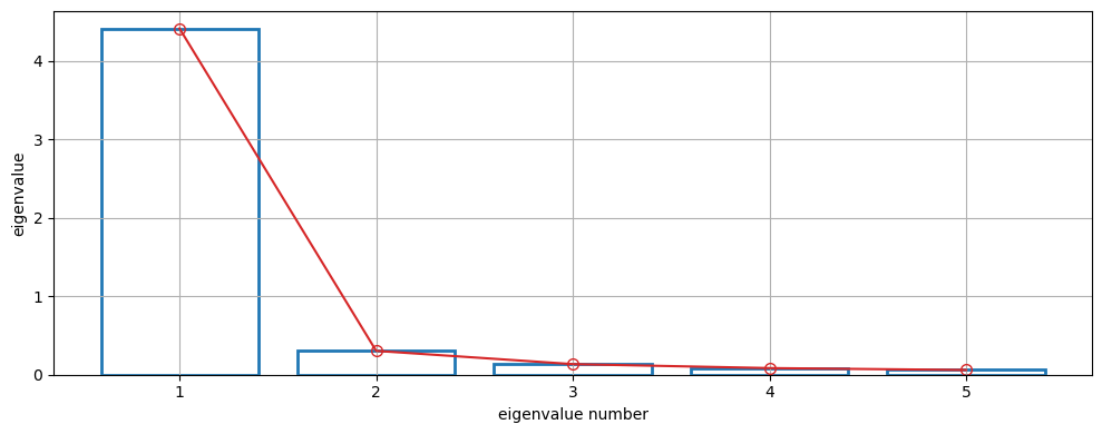
Scree plot

We can draw a scree plot to visualize the eigenvalues (used in determining the number of factors).

[6]:

# Plot eigenvalues in scree plot, see e.g. Fig 2 in JoH paper
ax = mt.plots.scree_plot()

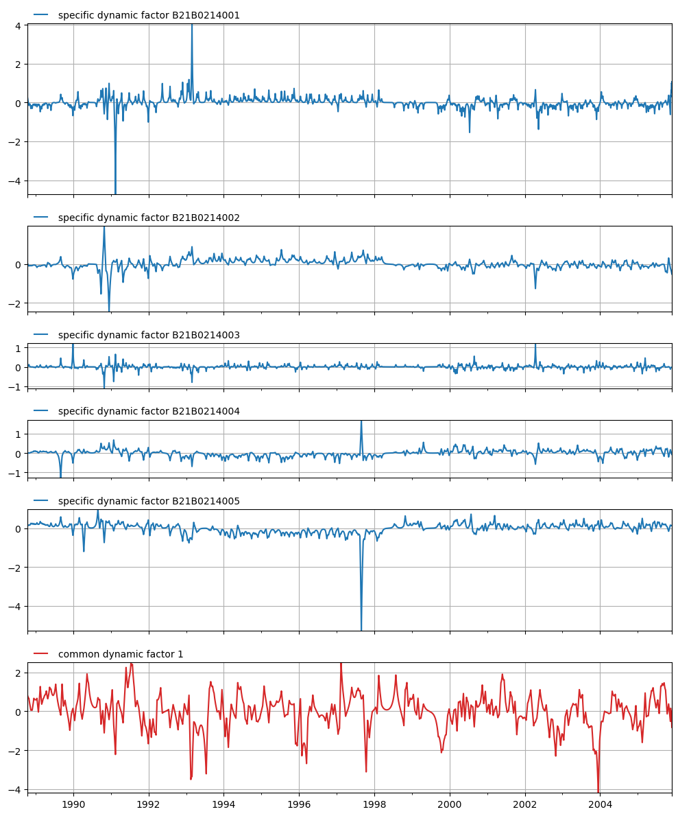
../_images/examples_ex01_metran_practical_example_10_0.png

State means

Plot the calculated state means for each of the specific and common dynamic components:

[7]:

mt.get_state_means()

[7]:

	B21B0214001_sdf	B21B0214002_sdf	B21B0214003_sdf	B21B0214004_sdf	B21B0214005_sdf	cdf1
date
1988-10-14	0.226549	0.021665	0.028548	0.026005	0.153683	0.809228
1988-10-15	0.182900	0.013039	0.026154	0.022935	0.149910	0.790042
1988-10-16	0.145313	0.004483	0.024958	0.020043	0.147006	0.772353
1988-10-17	0.112540	-0.004048	0.024904	0.017306	0.144954	0.756126
1988-10-18	0.083497	-0.012601	0.025990	0.014702	0.143742	0.741331
...	...	...	...	...	...	...
2005-11-24	0.909463	-0.389068	-0.022535	-0.002155	0.133346	-0.152090
2005-11-25	0.940340	-0.416086	-0.021679	-0.017868	0.134755	-0.288478
2005-11-26	1.001189	-0.445368	-0.021816	-0.033719	0.136945	-0.426332
2005-11-27	0.951887	-0.477072	-0.022951	-0.049831	0.139928	-0.675974
2005-11-28	1.068061	-0.511373	-0.025137	-0.066328	0.143722	-0.823190

6255 rows × 6 columns

[8]:

axes = mt.plots.state_means(adjust_height=True)

../_images/examples_ex01_metran_practical_example_13_0.png

Simulations

The simulated mean values for each time series in our Metran model can be obtained with:

[9]:

# Get all (smoothed) simulated state means
means = mt.get_simulated_means()
means.head(10)

[9]:

	B21B0214001	B21B0214002	B21B0214003	B21B0214004	B21B0214005
date
1988-10-14	5.450000	4.280000	4.620000	4.640000	5.480000
1988-10-15	5.094121	4.132049	4.500647	4.514891	5.348733
1988-10-16	4.781724	3.992287	4.396365	4.399175	5.231284
1988-10-17	4.505266	3.860280	4.306655	4.292536	5.127359
1988-10-18	4.258161	3.735609	4.231336	4.194678	5.036712
1988-10-19	4.034568	3.617869	4.170535	4.105327	4.959142
1988-10-20	3.829204	3.506668	4.124708	4.024229	4.894493
1988-10-21	3.637170	3.401621	4.094661	3.951149	4.842653
1988-10-22	3.453793	3.302355	4.081594	3.885870	4.803556
1988-10-23	3.274477	3.208502	4.087163	3.828191	4.777178

For obtaining the data for a simulation with the observations and an (optional) confidence interval, use mt.get_simulation().

[10]:

# Get simulated mean for specific series with/without confidence interval
name = "B21B0214005"
sim = mt.get_simulation(name, alpha=0.05)
sim.head(10)

[10]:

	mean	lower	upper
date
1988-10-14	5.480000	5.480000	5.480000
1988-10-15	5.348733	1.669956	9.027510
1988-10-16	5.231284	0.273555	10.189012
1988-10-17	5.127359	-0.640237	10.894955
1988-10-18	5.036712	-1.263478	11.336903
1988-10-19	4.959142	-1.669234	11.587519
1988-10-20	4.894493	-1.891043	11.680029
1988-10-21	4.842653	-1.942746	11.628053
1988-10-22	4.803556	-1.824438	11.431550
1988-10-23	4.777178	-1.522468	11.076824

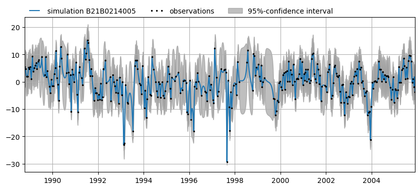
There is also a method to visualize these results for a single time series including optional confidence interval:

[11]:

ax = mt.plots.simulation("B21B0214005", alpha=0.05)

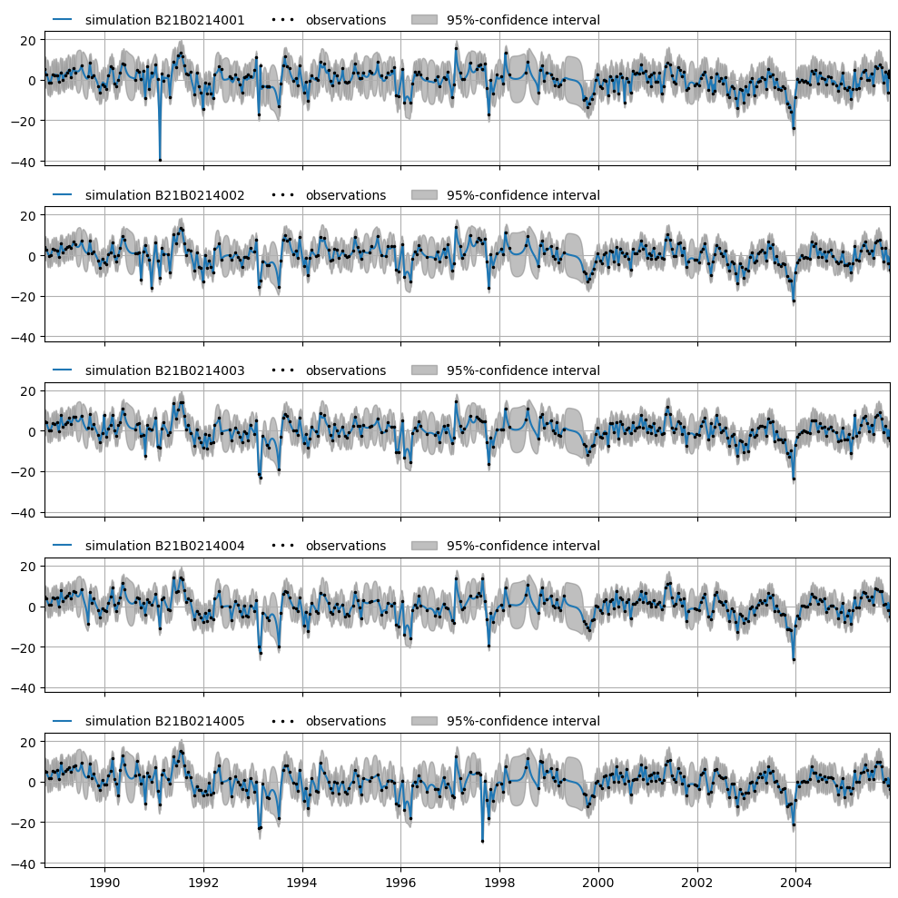
../_images/examples_ex01_metran_practical_example_19_0.png

Or all for all time series:

[12]:

axes = mt.plots.simulations(alpha=0.05)

../_images/examples_ex01_metran_practical_example_21_0.png

Decompositions

The decomposition of a simulation into specific and common dynamic components can be obtained with mt.decompose_simulation().

[13]:

# Decomposed simulated mean for specific series
decomposition = mt.decompose_simulation("B21B0214001")
decomposition.head(10)

[13]:

	sdf	cdf1
date
1988-10-14	1.339364	4.110636
1988-10-15	1.080942	4.013179
1988-10-16	0.858403	3.923322
1988-10-17	0.664372	3.840894
1988-10-18	0.492420	3.765741
1988-10-19	0.336849	3.697720
1988-10-20	0.192504	3.636701
1988-10-21	0.054601	3.582569
1988-10-22	-0.081428	3.535222
1988-10-23	-0.220092	3.494570

This can also be visualized:

[14]:

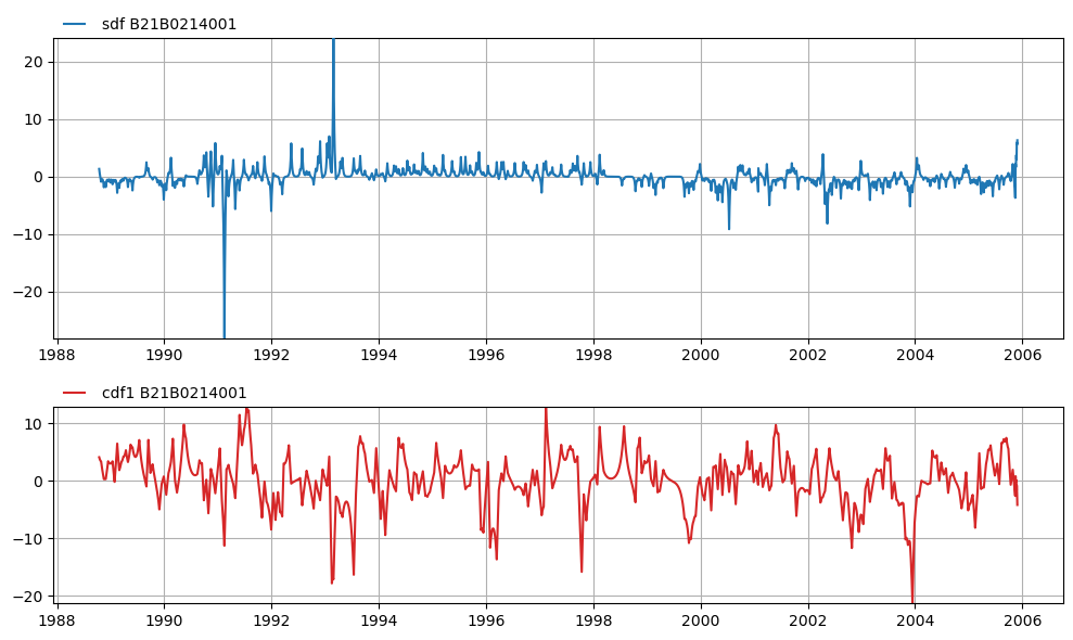
axes = mt.plots.decomposition("B21B0214001", split=True, adjust_height=True)

../_images/examples_ex01_metran_practical_example_25_0.png

Or for all time series

[15]:

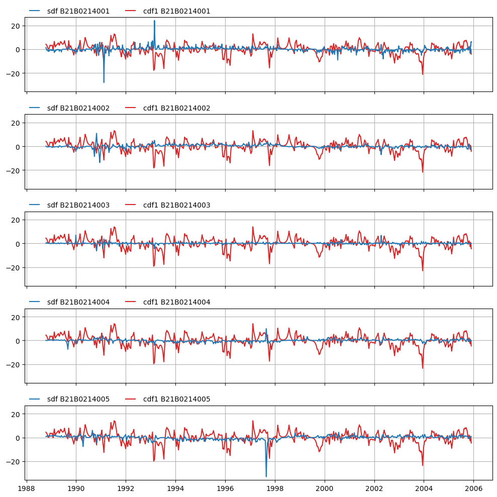
axes = mt.plots.decompositions()

../_images/examples_ex01_metran_practical_example_27_0.png

Example application: removing outliers

The Kalman smoother can be re-run after removing (masking) outliers from the observations. This is illustrated below.

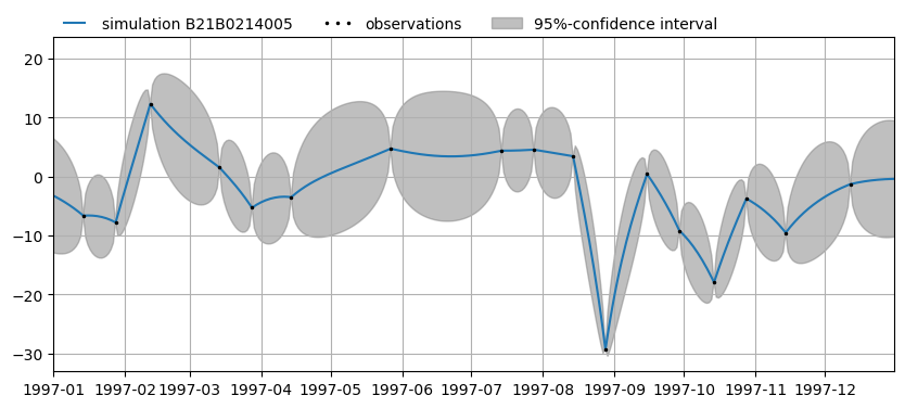
First plot the simulation for the original data:

[16]:

name = "B21B0214005"
alpha = 0.05

ax1 = mt.plots.simulation(name, alpha=alpha, tmin="1997-01-01", tmax="1997-12-31")

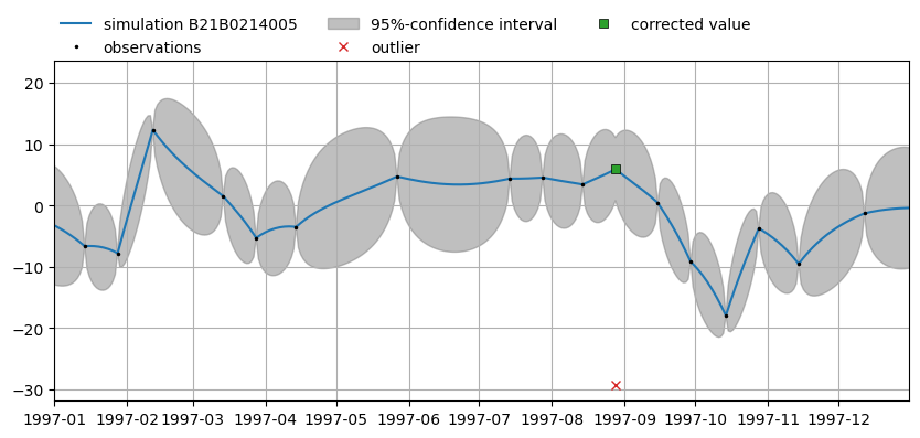
../_images/examples_ex01_metran_practical_example_29_0.png

Mask (remove) the outlier on 28 august 1997.

[17]:

oseries = mt.get_observations()
mask = (0 * oseries).astype(bool)
mask.loc["1997-8-28", name] = True
mt.mask_observations(mask)

Now plot the simulation again. Note the estimated value and its 95%-confidence interval for the observation on 28 August 1997 based on the common dynamic factor.

[18]:

# remove outlier from series B21B0214005 at 1997-8-28
# and re-run smoother to get estimate of observation
# (Fig 3 in Stromingen without deterministic component)
ax2 = mt.plots.simulation(name, alpha=alpha, tmin="1997-01-01", tmax="1997-12-31")
sim = mt.get_simulation(name, alpha=None).loc[["1997-8-28"]]

# plot outlier and corrected value
outlier = oseries.loc[["1997-8-28"], name]
ax2.plot(outlier.index, outlier, "C3x", label="outlier")
ax2.plot(sim.index, sim, "C2s", label="corrected value", mec="k", mew=0.5)
ax2.legend(loc=(0, 1), numpoints=1, frameon=False, ncol=3)

INFO: Running Kalman filter with masked observations.

../_images/examples_ex01_metran_practical_example_33_1.png

To reset the observations (remove all masks):

[19]:

# unmask observations to get original observations
mt.unmask_observations()

References

Van Geer, F.C. en W.L. Berendrecht (2015) Meervoudige tijdreeksmodellen en de samenhang in stijghoogtereeksen. Stromingen 23 nummer 3, pp. 25-36.