Pastas and Metran example

This notebook shows how output from Pastas time series models can be analyzed using Metran.

import os

import hydropandas as hpd
import matplotlib.pyplot as plt
import numpy as np
import pandas as pd
import pastas as ps

import metran

ps.logger.setLevel("ERROR")

metran.show_versions()

Python version: 3.10.12 | packaged by conda-forge | (main, Jun 23 2023, 22:40:32) [GCC 12.3.0]
numpy version: 1.26.4
scipy version: 1.12.0
pandas version: 2.0.3
matplotlib version: 3.8.3
pastas version: 1.4.0
numba version: 0.59.0
lmfit version: 1.2.2

Read data

Load the observed heads from piezometers at different depths at location B21B0214. The outliers (values outside of \(5 \sigma\) (std. dev.)) are removed from the time series.

oc = hpd.read_dino("./data", subdir=".")

oc

	x	y	filename	source	unit	monitoring_well	tube_nr	screen_top	screen_bottom	ground_level	tube_top	metadata_available	obs
name
B21B0214-001	198085.0	518413.0	B21B0214001_1	dino	m NAP	B21B0214	1.0	-7.3	-9.3	-0.29	0.24	True	GroundwaterObs B21B0214-001 -----metadata-----...
B21B0214-003	198085.0	518413.0	B21B0214003_1	dino	m NAP	B21B0214	3.0	-24.3	-26.3	-0.29	0.25	True	GroundwaterObs B21B0214-003 -----metadata-----...
B21B0214-002	198085.0	518413.0	B21B0214002_1	dino	m NAP	B21B0214	2.0	-15.3	-17.3	-0.29	0.28	True	GroundwaterObs B21B0214-002 -----metadata-----...
B21B0214-004	198085.0	518413.0	B21B0214004_1	dino	m NAP	B21B0214	4.0	-36.3	-38.3	-0.29	0.23	True	GroundwaterObs B21B0214-004 -----metadata-----...
B21B0214-005	198085.0	518413.0	B21B0214005_1	dino	m NAP	B21B0214	5.0	-51.3	-53.3	-0.29	0.21	True	GroundwaterObs B21B0214-005 -----metadata-----...

oseries = {}

for o in oc.obs:
    name = o.name
    o = o["stand_m_tov_nap"].rename(o.name)

    # remove outliers outside 5*std
    mean = o.median()
    std = o.std()
    mask_outliers = (o - mean).abs() > 5 * std

    ts = o.copy()
    ts.loc[mask_outliers] = np.nan

    # store time series
    oseries[name] = ts

# sort the names
sorted_names = list(oseries.keys())
sorted_names.sort()
sorted_names

['B21B0214-001',
 'B21B0214-002',
 'B21B0214-003',
 'B21B0214-004',
 'B21B0214-005']

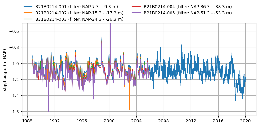
Plot the heads:

fig, ax = plt.subplots(1, 1, figsize=(10, 4))

for name in sorted_names:
    o = oseries[name]
    ftop = oc.loc[name, "screen_top"]
    fbot = oc.loc[name, "screen_bottom"]
    lbl = f"{name} (filter: NAP{ftop:+.1f} - {fbot:+.1f} m)"
    ax.plot(o.index, o, label=lbl)

ax.set_ylabel("stijghoogte (m NAP)")
ax.legend(loc=(0, 1), ncol=2, frameon=False)
ax.set_ylim(top=-0.5)
ax.grid(True)

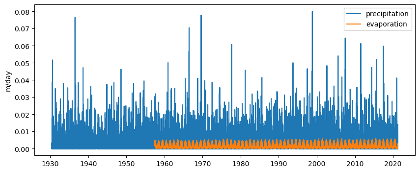
Load the precipitation and evaporation data from two nearby weather stations

p = pd.read_csv(
    "./data/RD_338.csv", index_col=[0], parse_dates=True, usecols=["YYYYMMDD", "RD"]
)
e = pd.read_csv(
    "./data/EV24_260.csv", index_col=[0], parse_dates=True, usecols=["YYYYMMDD", "EV24"]
)

Plot precipitation and evaporation time series

fig, ax = plt.subplots(1, 1, figsize=(10, 4))
ax.plot(p.index, p, label="precipitation")
ax.plot(e.index, e, label="evaporation")
ax.set_ylabel("m/day")
ax.legend(loc="best")

<matplotlib.legend.Legend at 0x7fe032f56770>

Build time series models

The time series models attempt to simulate the heads using recharge as stress. The recharge is calculated using \(R = P - f \cdot E\), where \(R\) is recharge, \(P\) is precipitation, \(E\) is evaporation and \(f\) is factor that is optimized. The model fit results are printed to the console. The model residuals are stored for analysis with Metran.

# Normalize the index (reset observation time to midnight (the end of the day)).
p.index = p.index.normalize()
e.index = e.index.normalize()

# set tmin/tmax
tmin = "1988-10-14"
tmax = "2005-11-28"

# store models and residuals
models = []
residuals = []

for name in sorted_names:
    # create model
    ml = ps.Model(oseries[name])
    rm = ps.RechargeModel(prec=p, evap=e)
    ml.add_stressmodel(rm)

    # solve model
    ml.solve(tmin=tmin, tmax=tmax, report=False)

    # print fit statistic
    print(name, f"EVP = {ml.stats.evp():.1f}%")

    # store model
    models.append(ml)

    # get residuals
    r = ml.residuals()
    r.name = name
    residuals.append(r)

B21B0214-001 EVP = 68.4%
B21B0214-002 EVP = 58.9%
B21B0214-003 EVP = 66.8%
B21B0214-004 EVP = 61.3%
B21B0214-005 EVP = 51.0%

Build Metran model

A Metran model is created using the residuals of the time series models. By analyzing the model residuals we can determine for example, whether there is a common pattern in the residuals, which could indicate a missing influence, or a shortcoming in the model structure. Additionally we might be able to analyze whether there are still outliers left in our time series.

mt = metran.Metran(residuals)
mt.solve()

INFO: Number of factors according to Velicer's MAP test: 1

Fit report Cluster                  Fit Statistics
======================================================
tmin     None                       obj       3223.12
tmax     None                       nfev            7
freq     D                          AIC       3235.12
solver   ScipySolve

Parameters (6 were optimized)
======================================================
                        optimal   stderr initial  vary
B21B0214-001_sdf_alpha       10  ±10.00%      10  True
B21B0214-002_sdf_alpha       10  ±10.00%      10  True
B21B0214-003_sdf_alpha       10  ±10.00%      10  True
B21B0214-004_sdf_alpha       10  ±10.00%      10  True
B21B0214-005_sdf_alpha       10  ±10.00%      10  True
cdf1_alpha                   10  ±10.00%      10  True

Parameter correlations |rho| > 0.5
======================================================
None

Metran report Cluster          Factor Analysis
==============================================
tmin     None                nfct      1
tmax     None                fep     81.32%
freq     D

Communality
==============================================

B21B0214-001      84.36%
B21B0214-002      67.77%
B21B0214-003      88.55%
B21B0214-004      90.71%
B21B0214-005      63.38%

State parameters
==============================================
                       phi         q
B21B0214-001_sdf  0.904837  0.028355
B21B0214-002_sdf  0.904837  0.058418
B21B0214-003_sdf  0.904837  0.020764
B21B0214-004_sdf  0.904837  0.016846
B21B0214-005_sdf  0.904837  0.066383
cdf1              0.904837  0.181269

Observation parameters
==============================================
                    gamma1     scale      mean
B21B0214-001      0.918464  0.052053 -0.000691
B21B0214-002      0.823243  0.060746 -0.000529
B21B0214-003      0.940984  0.050673 -0.000204
B21B0214-004      0.952399  0.056584  0.000345
B21B0214-005      0.796109  0.070582  0.000577

State correlations |rho| > 0.5
==============================================
None

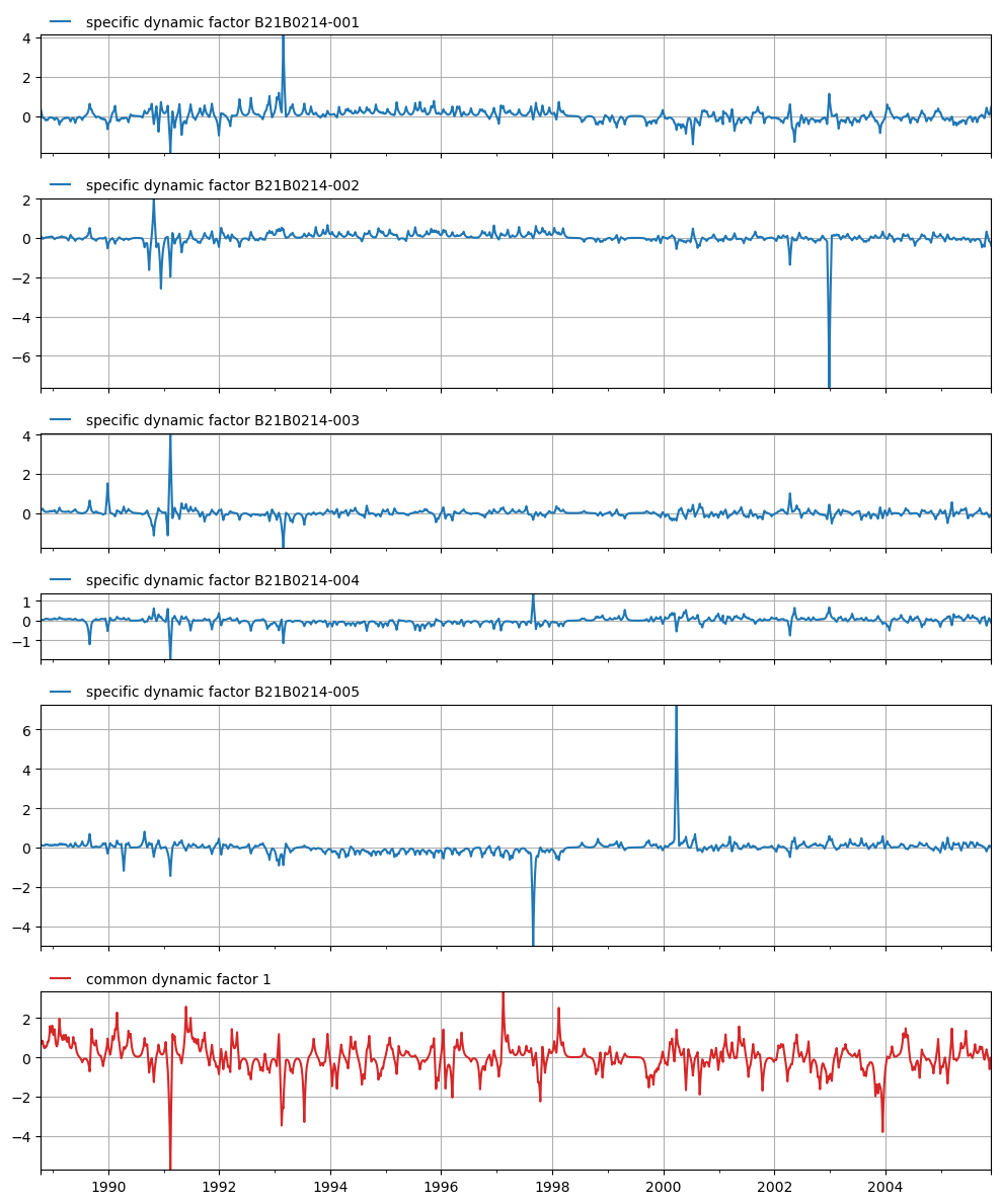
Plot the specific and common dynamic components

axes = mt.plots.state_means()

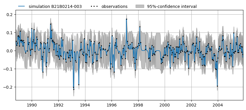
Plot a simulation, including a confidence interval for B21B0214003.

ax = mt.plots.simulation(mt.snames[2])